flowchart LR
  Mesh["Uniform Cartesian mesh"] --> Space["FiniteElementSpace"]
  Element["Element type"] --> Space
  Quad["Quadrature rule"] --> Space
  Space --> Assembly["Assembly: evaluateAx / evaluateLoadVector"]
13 Finite Elements
The Finite Element Method (FEM) is a way to solve partial differential equations which consists of meshing the domain with elements and approximating the solution on these elements. For an intro to FEM, see the following lecture notes, as well as the FEniCSx documentation, which shows how to discretize the Poisson equation with the Finite Element Method.
Typically, applying FEM to a PDE results in a linear system of equations to solve \[ A\mathbf{x} = \mathbf{b}, \] where \(A\) is known as the stiffness matrix and \(\mathbf{b}\) as the load vector. These vector contain values at locations known as degrees of freedom (DOFs), and are imposed by the finite element representation/space one chooses.
To solve a PDE, one can therefore choose a finite element discretization, and then solve the system \(A\mathbf{x} = \mathbf{b}\) with a method like Conjugate Gradient, given that \(A\) is symmetric positive definite.
In IPPL, the FEM framework can be found under src/FEM. It contains all the machinery to define quadratures, elements, finite element spaces, interpolation schemes, and degree-of-freedom storage. Currently, only structured Cartesian meshes with uniform mesh spacing are supported. Furthermore, only first-order Lagrange and Nédélec finite element spaces are available.
Ongoing work: higher-order finite element spaces, and implementation of Raviart-Thomas finite element space.
For information about finite element spaces and their implementation, please see https://defelement.org/.
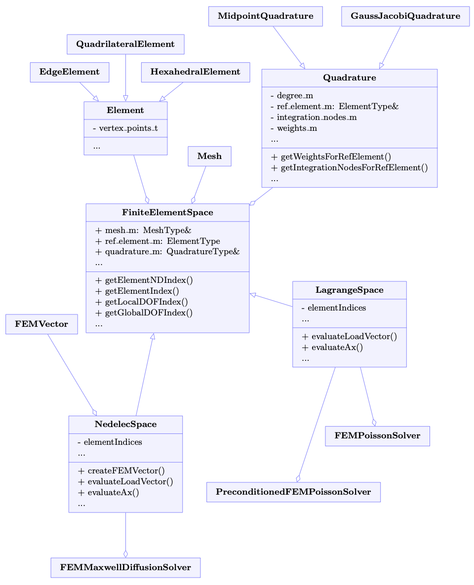
13.1 Main classes
| Class | Role |
|---|---|
FiniteElementSpace |
Common finite-element space base for structured rectilinear meshes and element indexing. |
LagrangeSpace |
Nodal Lagrange finite-element space for scalar fields. |
NedelecSpace |
Edge-oriented Nedelec finite-element space, to represent electric fields. |
FEMVector |
Data structure to store degrees of freedom. |
FEMInterpolate |
Interpolation operators from particles to FEM mesh (degrees of freedom) and vice versa. |
EdgeElement(1D), QuadrilateralElement (2D), HexahedralElement (3D) |
Reference element definitions. |
MidpointQuadrature, GaussJacobiQuadrature |
Integration quadrature definitions, based on different schemes. |
Currently, the FEMVector is the data structure to store degrees of freedom at arbitrary locations. It is used in the NedelecSpace to store the edge degrees of freedom. However, in the first-order Lagrange case, degrees of freedom exist only at vertices i.e. they are confounded with the nodal grid. Hence, in LagrangeSpace, we use the normal IPPL fields and meshes to store the degree of freedom data. This should be changed to adopt the FEMVector or other alternative degree of freedom storage solutions for higher-order Lagrange spaces, where degrees of freedom can exist on edges and faces too.
To interface the FEM framework into Particle-Mesh methods, in particular Particle-in-Cell, one also needs an appropriate interpolation to and from the finite element space for the scatter and gather in the PIC loop (see Chapter 3). This is provided by FEMInterpolate.
13.2 Space construction
A finite-element calculation starts from the same distributed mesh concepts used by fields: a mesh, a domain, and a layout. The FEM space adds an element, a reference element, and a quadrature rule. The space is then responsible for mapping mesh vertices to elements, local DOFs to global DOFs, and evaluating the load vector \(\mathbf{b}\) as well as the matrix-vector product \(A\mathbf{x}\).
13.3 Lagrange space
LagrangeSpace represents structured-grid nodal Lagrange elements, and is templated on the order. The number of element DOFs is computed as (Order + 1)^Dim. It uses IPPL fields to store the degrees of freedom, since in the first-order case these are confounded with mesh vertices.
The class exposes the pieces a user expects to solve a given PDE:
| Capability | Use |
|---|---|
| Basis and gradient evaluation | Evaluate shape functions and derivatives at quadrature points. |
evaluateAx |
Apply the action of the stiffness matrix A on a vector x without assembling the full matrix - this is a matrix-free operator. |
evaluateLoadVector |
Assemble the load vector from a given right-hand side. |
computeErrorL2 |
Compute the relative error with respect to a given analytical function. |
updateLayout |
Update the finite element distribution if the layout changes due to new domain decomposition via load balancing. |
evaluateAx takes in a functor which represents the weak form of the equation we want to solve.
Currently, Lagrange space supports Zero BCs, Dirichlet BCs, and Periodic BCs.
N.B. Only first-order supported currently.
13.4 Nedelec space
NedelecSpace provides vector-valued edge DOFs, used to represent electric fields in the Maxwell equations.
It uses the FEMVector as its degree of freedom storage, as opposed to IPPL fields (like the LagrangeSpace). The FEMVector is a flat one-dimensional Kokkos::View<T*>, whose indices need to be mapped to the elements and their degrees of freedom.
| Capability | Use |
|---|---|
| Basis and curl evaluation | Evaluate vector basis functions and their curls. |
getFEMVectorDOFIndices |
Map FEM vector entries to local element DOFs. |
evaluateAx |
Apply FEM matrix to a vector (given a weak form of a PDE). |
evaluateLoadVector |
Build the load vector given a right-hand side. |
createFEMVector |
Construct the FEMVector for DOF storage. |
Currently, Nédélec space supports only Zero BCs.
N.B. Only first-order supported currently.
13.5 Unit tests
| Test family | Manual purpose |
|---|---|
unit_tests/FEM/FiniteElementSpace.cpp |
Validate element indexing and local/global DOF mapping. |
unit_tests/FEM/LagrangeSpace.cpp |
Validate scalar basis functions and assembly. |
unit_tests/FEM/NedelecSpace.cpp |
Validate edge basis functions, curls, and vector DOF mapping. |
13.6 Matrix-free FEM-based solver workflow
In order to create FEM-based solver, one needs to use the Finite Element spaces with a given PDE.
The general steps to solve a PDE using FEM given a space are the following:
- Build the load vector using the right-hand side by calling
evaluateLoadVector. - Define a functor which represents the weak form of the PDE we seek to solve on the reference element, e.g.
weak_form(). - Given this functor, we can evaluate the matrix-vector product \(A\mathbf{x}\) in a matrix-free manner, calling
evaluateAx(weak_form). - Solve iteratively using (Preconditioned) Conjugate Gradient – only if the matrix is symmetric positive definite. The Conjugate Gradient method can be found in
src/LinearSolvers, and requires a matrix-vector operator to use it. Hence, we pass to it an operator which callsevaluateAx(weak_form). - Obtain the solution from the iterative solver.
For example, we can solve the Poisson equation, which has the following weak form: \[
\int_{\Omega} \nabla \phi \cdot \nabla v = \int_{\Omega} \rho \cdot v, \hspace{4mm} \forall v \in V_h,
\] where \(\phi\) is the solution we are looking for, \(\rho\) is the source (right-hand side), and \(v\) is known as the test function, and \(V_h\) the test space (Finite Element space). Typically we look for the solution in the same space as the test space (Galerkin finite element method). Typically, one can use the Lagrange space to solve the Poisson equation. In IPPL, the FEM-based Poisson solver can be found in src/PoissonSolvers/FEMPoissonSolver.h.
One can also solve the electromagnetic diffusion problem using the Nédélec space to represent the electric field: \[
\begin{align}\label{eq:diffusion}
\nabla \times \nabla \times \vec{u}(\vec{x}) + \vec{u}(\vec{x}) &= \vec{g}(\vec{x}) \text{ in } \Omega,\\
\vec{u}(\vec{x}) \times \vec{n} &= \vec{0} \text{ on } \partial \Omega\text{,}
\end{align}
\] where \(g\) is a source function, \(\mathbf{n}\) is a normal vector pointing outwards from the surface, and \(u\) is the solution we seek. This can be found in src/MaxwellSolvers/FEMMaxwellDiffusionSolver.h.
13.7 Boundary and layout handling
- Element ownership: Each rank owns a set of elements and is responsible for them. The rank ownership is determined at the creation of the Finite Element space: given a layout and a domain decomposition the elements are distributed accordingly. If doing dynamic load balancing during the simulation, one can call the
updateLayout()function of the space in order to update the element distribution among ranks. - Halo cells: Halo cells are necessary to enforce correctness given a distributed mesh, since elements share degrees of freedom with neighbouring ranks. Furthermore, these also help enforce boundary conditions.
13.8 FEM-PIC coupling in practice
For electrostatic PIC with FEM Poisson, scatter/gather is replaced by basis-function projections:
- Particle-to-mesh: assemble load vector from particle charges evaluated through FEM basis functions.
- Mesh-to-particle: interpolate solved DOF values back to particle positions.
These interpolations are present in src/FEM/FEMInterpolate.h.
The FEM-based poisson solver, src/PoissonSolvers/FEMPoissonSolver.h, is available as a solver in the alpine/LandauDamping.cpp PIC mini-app. This makes use of the FEM-based interpolation in the scatter/gather steps.