flowchart TB
  User["Application or mini-app"]
  Manager["Manager layer"]
  Particle["Particle containers"]
  Field["Distributed fields"]
  FieldSolver["Field solvers"]
  Mesh["Mesh, index, region"]
  Interp["Interpolation"]
  Solver["Poisson, Maxwell"]
  Comm["MPI communication"]
  Kokkos["Kokkos execution and memory spaces"]
  Heffte["HeFFTe FFT backend"]

  User --> Manager
  Manager --> Particle
  Manager --> Field
  Manager --> FieldSolver
  Particle --> Interp
  Interp --> Field
  Field --> Mesh
  FieldSolver --> Solver
  Solver --> Field
  Solver --> Heffte
  Particle --> Comm
  Field --> Comm
  Comm --> Kokkos
  Field --> Kokkos
  Particle --> Kokkos
2 Overview
IPPL provides reusable components for scientific simulations that need distributed fields, particles, interpolation, FFTs, and solvers. The library is designed around templates for dimension, floating point precision, and execution space, so the same user code can target serial, OpenMP, CUDA, or HIP builds when the backend stack is available.
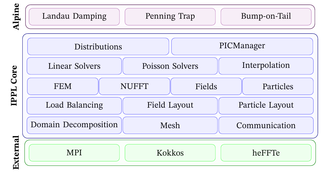
IPPL has a modular interface, containing all the building blocks of particle-mesh simulations which can be mixed and matched. For example, it is possible for users to only use the part of the library they need, such as field solvers to solve the Poisson equation, without having to use particles or go through a PIC style simulation. Furthermore, these building blocks are written in a dimension independent manner, supporting the same number of dimensions as supported by Kokkos views (see Kokkos documentation). IPPL has full Particle-in-Cell capabilities for 1D, 2D, and 3D simulations. One can choose the floating point precision of many of the components, making it simple to run mixed precision simulations.
On top of the IPPL core, we have Alpine. This is a set of benchmark applications from plasma physics, such as Landau damping or a Penning trap, which are used to verify correctness as well as measure performance [1]. Furthermore, these provide an example for how to use IPPL on an application level, to simulate physical plasmas in this case. These mini-apps are introduced in Chapter 5.
2.1 Main capabilities
| Area | Primary IPPL components |
|---|---|
| Runtime environment | ippl::initialize, ippl::finalize, ippl::Comm, ippl::Info |
| Geometry and indexing | Index, NDIndex, NDRegion, PRegion, UniformCartesian |
| Distributed fields | BareField, Field, FieldLayout, halo cells, boundary conditions |
| Particles | ParticleBase, ParticleAttrib, spatial layouts, migration |
| Particle-mesh coupling | CIC, gather, scatter, PIC manager patterns |
| Spectral methods | FFT, HeFFTe backends, Poisson solvers |
| PDE solvers | FFT Poisson, FEM Poisson, Maxwell FDTD, linear solvers |
| Portability | Kokkos execution spaces, mixed precision, GPU-aware MPI |