9 Interpolation in Particle-Mesh methods
Particle-mesh workflows combine distributed particles, distributed fields, interpolation, and solvers. The core cycle is common across plasma, accelerator, and astrophysical applications. More concretely, it is the basis of the Particle-in-Cell (PIC) method introduced in Chapter 3.
As a reminder, the core operations of a Particle-Mesh method result from the intertwining of a Lagrangian and Eulerian approach. In the case of the PIC method, these operations form the PIC loop:
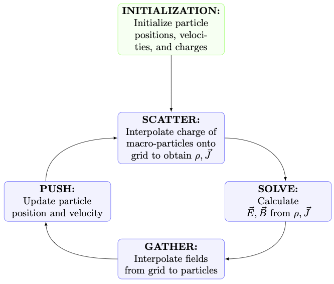
The scatter and gather operations in the PIC loop (see Chapter 3) require interpolation from particles to grid and vice-versa. The choice of interpolation scheme depends on the accuracy needs of the application.
9.1 CIC interface
Cloud-in-Cell (CIC) interpolation is a first-order method which distributes a particle attribute among all the surrounding grid points according to the distance between the particle and the points.
Currently, CIC interpolation can be applied to a particle attribute by using global gather/scatter functions defined in src/Interpolation/CIC.h. The implementation scatters to or gathers from 2^Dim neighboring mesh points. In 2D, for example, the contributing points are (i, j), (i - 1, j), (i, j - 1), and (i - 1, j - 1).
The example below scatters the charge-to-mass ratio qm from particles to the rho field on the grid, and gathers back the electric field efield to the particle positions:
scatter(qm, rho, bunch.R);
gather(bunch.E, efield, bunch.R);
As can be seen, both the scatter and gather calls function for scalar fields (like rho) and vector fields (like efield).
9.2 CIC weights and conservation
For each particle, CIC computes lower and upper interpolation weights in every dimension. Scatter uses atomic adds into the field:
Kokkos::atomic_add(&field(...), particleValue * weightProduct);Gather computes the weighted sum of the same neighboring mesh points.
The particle gather/scatter tests verify the following operations:
| Test | Expected behaviour |
|---|---|
| Gather from constant field | Interpolation of a constant field returns that constant. |
Gather with addToAttribute = false/true |
Gathered values can either replace or increment an attribute. |
| Scatter all charged particles | Total field charge equals total particle charge. |
| Scatter with custom range | A subset of local particles can be deposited. |
| Scatter with custom hash | Particles can be deposited through a remapped index list. |
Typical calls:
field = 0.0;
scatter(bunch.Q, field, bunch.R);
double totalField = field.sum();
double totalParticles = bunch.Q.sum();

gather(bunch.Q, field, bunch.R);
gather(bunch.Q, field, bunch.R, true); // addToAttribute=true
9.3 PIC test loop
The PICnd test exercises the following end-to-end sequence:
- Construct
NDIndex,UniformCartesian,FieldLayout, andParticleSpatialLayout. - Create a derived
ParticleBasecontainer and register particle attributes. - Initialize particle positions and attributes.
- Call
update()to migrate particles to owning ranks. - Deposit particle charge with
scatter. - Initialize a static electric field.
- Gather the electric field at particle locations with
gather. - Advance particle velocity and position.
- Repeat migration and conservation checks.
The time loop in PICnd has the canonical PIC shape (in the electrostatic case):
bunch->R = bunch->R + dt * bunch->P;
bunch->update();

bunch->scatterCIC();
bunch->gatherCIC();

bunch->P = bunch->P + dt * bunch->qm * bunch->E;
The position is updated using the particle velocities, then update is called to make sure particles are in the correct rank. Then, we call scatterCIC to scatter from particles to grid using CIC interpolation. This would be followed by a solve step to solve for the electric field using the charge density, in the case of an electrostatic PIC simulation. However, this step is skipped in this test, since it seeks to test only the interpolation. Next, the gatherCIC interpolates the electric field back to particle positions, populating bunch->E. Finally, the velocities are updated using the computed electric field and the charge-to-mass ratio (electrostatic Lorentz force).
scatterCIC resets the mesh field, deposits charge, reduces the total particle count, and checks charge conservation:
EFDMag_m = 0.0;
scatter(qm, EFDMag_m, this->R);

double Q_grid = EFDMag_m.sum();
ippl::Comm->reduce(&local_particles, &Total_particles, 1, std::plus<unsigned int>());
double rel_error = std::fabs((this->Q_m - Q_grid) / this->Q_m);
The PICnd test can be run using the following command line shape:
srun ./PICnd 128 128 128 10000 10 --info 10where the first three arguments are grid sizes (in 3D), followed by total particle count and number of time steps. In the above case, we are running a \(128^3\) grid size with 10000 particles for 10 time steps.
9.4 Load balancing
PICnd also shows a first load-balancing pattern. It initializes an OrthogonalRecursiveBisection object using the field layout, mesh, and field magnitude. During the simulation, the domain can be repartitioned according to the particle positions:
orb.initialize(fl, mesh, EFDMag_m);

...

bool changed = orb.binaryRepartition(this->R, fl);
if (changed) {
    this->updateLayout(fl, mesh);
}
The important user contract is that field layouts, local fields, and particle layouts must be updated together after repartitioning.
9.5 First examples to document
TODO
test/particle/PICnd.cppfor a compact PIC test.alpine/LandauDamping.cppand ALPINE managers for production-style mini-apps.examples/collisions/P3MHeating.cppfor P3M-style coupling.